Mfr Part # ADS8668IDBTR
IC ADC 12BIT 38-TSSOP
Texas Instruments
License: Attribution Hall Effect Magnetic Magnets Solder / Desoldering Test Equipment ESP32
This project uses magnetic Hall effect sensors to accurately track the position of a magnet as it moves along a single axis. Multiple Hall effect sensors are chained together and placed along the magnet’s path to record its current location. The goals of the project are:
Tracking: The magnet’s position should be tracked reliably and within about 0.5 cm of accuracy when the magnet is moving linearly approximately 1 in away from the sensors.
Adaptability: The final device must be daisy-chainable. In other words, the PCB designed to house the sensors should be able to link with other identical PCBs. This allows the device to adapt to changes in the length of the path that the magnet will travel along.
This project was made to support the goals of Space Enterprise at Berkeley, UC Berkeley’s liquid rocketry team. This device will be integrated into the fuel tank on our test stand and will record fuel fill level by tracking the position of a piston, which will rise with fuel level. Magnets will be embedded in the piston to achieve this.
Read more about this in the Magnetic Fill Level Sensing in Liquid Bipropellant Rocketry section below. Learn more about Space Enterprise at Berkeley here.
DRV5055
This is a Hall effect sensor. It provides an output voltage that changes linearly in response to changes in magnetic flux density. Linked here.
ADS8668
This is an 8-channel 12-bit resolution analog-to-digital converter that will convert the analog output from the DRV5055 sensors to a digital reading. Linked here.
The high number of channels means fewer ADCs need to be used for the same number of sensors, lowering cost, simplifying part count, and easing development.
The high resolution means small changes in the DRV5055’s output voltages can be read
These ADCs are daisy-chainable and can be linked to one another
Magnets
I am using these 1/2 x 1/4 Inch N52 Neodymium Disc Magnets. Any magnet would work, but I chose them for their strength and relatively small size. Linked here.
Microcontroller
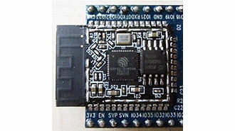
I am using the ESP-WROOM-32 Development Board for this project, but any microcontroller that supports SPI communication will work.
As the name suggests, Hall effect sensors take advantage of the Hall effect. They contain a current-carrying conductor that, when exposed to a magnetic field, develops a voltage across it (What is a Hall Effect Sensor?). The magnitude of this voltage is proportional to the magnetic flux density, or the strength of the magnetic field passing through the sensing element. This will increase as a magnet nears the sensor since the field is stronger closer to the magnet.
Texas Instruments’ DRV5055 sensors are designed to output this analog voltage, and this relationship is shown in the graph below. Magnetic field lines have a direction, and these sensors only sense the magnetic field component that is perpendicular to the top of the package. This is represented by vector B in the diagram below. In other words, the orientation of the sensor matters.
Photo credit: Texas Instruments DRV5055 datasheet
To show how the DRV5055 Hall effect sensors respond to magnets, we supplied them with 5 volts using a benchtop power supply and measured their output on a multimeter.
I 3D printed a sled to hold the magnet and a rail for it to slide along, emulating the movement of the magnet within the piston as it rises in the fuel tank. This was held together on a laser-cut wooden base.
Starting the magnet in line with the sensor and moving it away in increments of 2 cm, we found that the output voltage of the sensor changed proportionally to the magnet’s distance from it.
Multiple DRV5055 sensors produced identical results. The voltage drops as the magnet nears the sensor. If the magnet’s North and South poles were switched, the voltage would increase instead.
A thin sheet of aluminum in between the sensor and magnet mimics the wall of the fuel tank, which will separate the two. As expected, the non-magnetic aluminum has zero effect on the sensor output.
⚠️‼️I continued with the sensor oriented as shown above. This worked well, but an alternative orientation may have worked better, though requiring more computation to determine magnet position. See the Hall Effect Sensor Orientation section below.
Next, I designed a PCB to “break out” the pins on the ADS8668 and test its ability to interface with the DRV5055 sensors. This is a development board that mimics the final product in every way except in form factor. It also provides additional flexibility to change electrical connections and probe the pins on the ADC.
The board was designed in Altium Designer, with components sourced separately from DigiKey.
I assembled the board as shown below, attaching the SMD passives with solder paste and hand-soldering the through-hole DRV5055s and female header.
The female header allows for electrical connections between the board and microcontroller to be changed quickly, easing debugging and enabling the board to be tested standalone and in daisy-chain configuration.
To communicate with the development board, I used the PlatformIO IDE on VSCode. This plugin makes it easy to configure and interface with microcontrollers. Learn more about PlatformIO and how to use it here.
Photo credit: mischianti.org
To interface with the ADS8668 ADC, I used a public library found online by Github user siteswapjuggler. The library can be found here. This library is made for the ADS8688, which is identical to the ADS8668 but has 16-bit resolution instead of 12-bit resolution.
⚠️‼️Some changes I had to make in the library code were:
Change the SPI Mode from Mode 0 to Mode 1 (The ADS8668 uses SPI Mode 1). Additional info on SPI Interface and its four modes can be found here.
I added an init() function to initialize the ADC within the setup() function in the code. However, functioning code should be writable with just the library’s constructor.
The code I used to configure the ESP-WROOM-32 in the “platformio.ini” file is shown below. “magfill-adc-dev” is the folder that contains my “main.cpp” file with the code.
[env:magfill-adc-dev]
platform = espressif32
board = esp32dev
framework = arduino
monitor_speed = 115200
build_src_filter = -<*> +<tests/magfill-adc-dev/*>
The ADS8668 contains programmable registers that define its behavior. To read the DRV5055 sensors’ outputs through the ADC, I programmed each channel to operate at the input range of 0V to 1.25 x Vref (I used the chip’s internal 4.096-V reference). This code utilizes the ADS8688 library’s functions and is shown below.
#include <Arduino.h>
#include <ADS8688.h>

SPIClass *spi;
ADS8688 adc;				       //construct the ADS8688 object

void setup() {
  spi = new SPIClass(HSPI);	       //create a SPI object
  spi->begin(18, 19, 23, 5);          //define SPI pins (based on microcontroller pinout)
  adc.init(spi, 27);			 //initialize ADC with the SPI object & CS pin
  adc.cmdRegister(RST);
  adc.setChannelSPD(0b11111111);
  adc.setGlobalRange(R6);             // set 0 to 1.25 x Vref range for all channels
  adc.autoRst();                      // reset auto channel switching
  Serial.begin(115200);
  pinMode(27, OUTPUT);

}

void loop() {
  Serial.print("values: ");               // print label
  for (byte i=0;i<8;i++) {
    uint16_t val = adc.noOp();            // trigger samples
    Serial.print(adc.I2V(val,R6));        // print value in Volts
    Serial.print(i !=7 ?" V | ":" V\n");  // print Volt label
  }
  delay(500);                             // wait for 500 milliseconds
  }
Note that SPIClass is included in the PlatformIO extension’s Arduino framework packages. This code takes inspiration from the ADS8688 library’s example code.
I connected the ESP to my development board via jumper wires, using both the ESP’s 3.3V and an external 5V power supply to power the board. 5V powered the DRV5055s and ADS8668’s analog input while 3.3V powered the ADS8668’s digital input.
After ensuring the power supply was stable and fixing some on-board electrical connections, I read the appropriate values from the development board on the serial monitor.
To calculate the magnet’s position based on the voltage outputs of the DRV5055 sensors:
Sum the readings of each pair of adjacent sensors.
Determine which pair has the lowest sum. Since the output voltage of each DRV5055 drops as the magnet nears it, the pair with the lowest sum must be the pair that the magnet is between.
Subtract the output of the second sensor in the pair from the output of the first sensor. This difference will be proportional to the magnet’s distance from the midpoint between the two sensors.
Difference = 0 : The magnet is exactly in between the two sensors
Difference < 0: The magnet is closer to the first sensor in the pair
Difference > 0: The magnet is closer to the second sensor in the pair
Scale this difference to determine the magnet’s exact distance from the midpoint.
Since the location of each sensor is known, and the magnet’s distance from a particular sensor is now known, the magnet’s position is known.
To determine the scaling factor ⍺ needed to scale the output difference to the distance of the magnet from the midpoint, I used the following equation:
I placed the magnet 0.5 cm to the right of the midpoint between two sensors. Using d = 0.5 as a constant and measuring the outputs of Sensor A and Sensor B, I calculated ⍺. I calculated ⍺ with three pairs of sensors and used the average of the results, determining ⍺ = 5.464.
I modified the code to implement this algorithm, as shown below. Because the channel numbers on the ADS8668 did not map to the order of the DRV5055s I placed physically on the board, I created an array mapOrder[] to remap them so the sensor readings correctly show in sequence.
#include <Arduino.h>
#include <ADS8688.h>

SPIClass *spi;
ADS8688 adc;

void setup() {
  spi = new SPIClass(HSPI);
  spi->begin(18, 19, 23, 5);
  adc.init(spi, 27);
  adc.cmdRegister(RST);
  adc.setChannelSPD(0b11111111);
  adc.setGlobalRange(R6);
  adc.autoRst();
  Serial.begin(115200);
  pinMode(27, OUTPUT);
}
//everything above this line is the same as before

uint8_t mapOrder[] = {2, 3, 4, 5, 6, 7, 0, 1}; double values[] = {-1, -1, -1, -1, -1, -1, -1, -1};
double minValue;
int minSense;
double zeroDistance = 0.35;     //location of first sensor
double a = 5.464;               //constant multiplier
double distance;                //Distance of magnet from
double spaceDistance = 2.54;    //Distance between sensors

void loop() {
  for (byte i=0; i<8; i++) {
    uint16_t val = adc.noOp();              // trigger samples
    values[mapOrder[i]] = adc.I2V(val,R6);
  }

  minSense = 0;
  minValue = values[0] + values[1];
  for (byte i=1; i<7; i++) {
    if (values[i] + values[i+1] < minValue) {
      minValue = values[i] + values[i+1];
      minSense = i;
  }

  distance = zeroDistance + spaceDistance*minSense + (spaceDistance / 2) + a*(values[minSense] - values[minSense+1]);

  for (byte i=0; i<8; i++) {
    Serial.print(values[i], 3);
    if (i < 7) {
      Serial.print(" V | ");
    }
    else{
      Serial.print(" V | minSense: ");
      Serial.print(minSense);
      Serial.print(" position: ");
      Serial.print(distance);
      Serial.print(" cm\n");
    }
  }
  delay(500);
}
Connecting the ESP to a development board and uploading the code, I moved a magnet along a custom 3D-printed rail while printing the calculated sensor position. It worked wonderfully, updating as the magnet moved along the board’s length.
Along most of the track, the calculated position is within about 0.5 cm of the magnet’s actual position. However, the DRV5055s do not all output the exact same voltage when no magnet is present, leading to some offsets in their output voltages. This introduces additional error, but the calculated position is still within about 1 cm of the magnet’s actual position when it’s near these sensors. Plans to resolve these issues are described in the Future Improvements section below. This will include zeroing the sensors so they share the same baseline.
Next, I added additional code to allow multiple ADS8668s to chain together. These ADCs function such that the output from one ADC can be passed to another by configuring them as shown below.
Photo credit: Texas Instruments ADS866x Datasheet
All ADCs receive the same input from the microcontroller, but the microcontroller must “listen” for longer to receive the outputs from all ADCs in the chain. It will receive the readings from the ADC closest to it, then the next, and so on. I added the following readDaisyChain function to the ADS8688 library.
void ADS8688::readDaisyChain(uint16_t *rawValues, int numADCs) {
    _theSPI->beginTransaction(SPISettings(1000000, MSBFIRST, SPI_MODE0));
    digitalWrite(_cs, LOW);

    _theSPI->transfer(0x00); //equivalent to sending 0x00 (NO_OP)
    _theSPI->transfer(0x00);

    // Read N 16-bit results (MSB first from ADC_N to ADC_1)
    for (int i = 0; i < numADCs; i++) {
        byte MSB = _theSPI->transfer(0x00);
        byte LSB = _theSPI->transfer(0x00);
        rawValues[i] = (MSB << 8) | LSB;
    }

    digitalWrite(_cs, HIGH);
    _theSPI->endTransaction();
    //return;
}
The for loop holds CS low for an additional 16 bits for every ADC that is added to the chain, accounting for the additional data transfer. A Normal Operation command is sent each time the CS pin is brought low to indicate no change in register programming.
A rawValues array temporarily holds the readings from each ADC. I altered the loop() function to adopt readDaisyChain and adapt to a larger number of total sensors. This new loop(), as well as additional variable declarations, can be seen in the modified code below.
#include <Arduino.h>
#include <ADS8688.h>

SPIClass *spi;
ADS8688 adc;

void setup() {
  spi = new SPIClass(HSPI);
  spi->begin(18, 19, 23, 5);
  adc.init(spi, 27);
  adc.cmdRegister(RST);
  adc.setChannelSPD(0b11111111);
  adc.setGlobalRange(R6);
  adc.autoRst();
  Serial.begin(115200);
  pinMode(27, OUTPUT);
}

double minValue;
int minSense;
double zeroDistance = 0.35;
double a = 5.464;
double distance;
double spaceDistance = 2.54;
//everything above this line is the same as before

uint8_t mapOrder[] = {2, 3, 4, 5, 6, 7, 0, 1, 10, 11, 12, 13, 14, 15, 8, 9};
double values[] = {-1, -1, -1, -1, -1, -1, -1, -1, -1, -1, -1, -1, -1, -1, -1, -1};
uint16_t rawValues[2];                //array to hold raw output from the ADC
int numADCs = 2;                      //number of ADCs in the chain

void loop() {
  Serial.print("values: ");
  for (byte i=0; i<8; i++) {
    adc.readDaisyChain(rawValues, numADCs);           // trigger samples
    for (int j=0; j<numADCs; j++) {
      values[mapOrder[i + 8*j]] = adc.I2V(rawValues[j],R6);
    }
  }

  minSense = 0;
  minValue = values[0] + values[1];
  for (byte i=1; i<(numADCs*8)-1; i++) {
    if (values[i] + values[i+1] < minValue) {
      minValue = values[i] + values[i+1];
      minSense = i;
    }
  }

  distance = zeroDistance + spaceDistance*minSense + (spaceDistance / 2) + a*(values[minSense] - values[minSense+1]);

  for (byte i=0; i<(numADCs*8); i++) {
    Serial.print(values[i], 3);
    if (i < (numADCs*8)-1) {
      Serial.print(" V | ");
    }
    else{
      Serial.print(" V | minSense: ");
      Serial.print(minSense);
      Serial.print(" position: ");
      Serial.print(distance);
      Serial.print(" cm\n");
    }
  }

  delay(500);
}
I tested this with two development boards and successfully read the sensor outputs from both. This setup and the serial monitor output are shown below.
Note that the two 0.00 readings are caused by faulty sensors. I probed the sensors directly and found that they outputted negative voltage, indicating broken internal circuitry. Replacing these would produce the correct readings and calculated position.
Some improvements that I will implement and that you should consider if you embark on a similar project are:
The formula that scales sensor output to magnet position is linear, while the actual relationship is not. Additional characterization can be done to produce a more accurately calculated position.
The sensors can be zeroed upon power-on of the device to establish a shared baseline. For about 5 to 10 conversion cycles, each sensor’s output values will be documented automatically. The average of these values will be calculated and used to offset each sensor’s readings so that they all share a common baseline or zero point.
At the start of this article, I briefly mentioned the motivation behind designing this device. I will now elaborate on the problem this was made to solve. This should both provide context and give inspiration as to what it can be used for.
Space Enterprise at Berkeley is a student team at UC Berkeley that develops liquid bipropellant rockets. A basic liquid bipropellant system consists of three tanks. Two primary tanks hold the two liquid propellants: The fuel and oxidizer. These mix together and combust to create thrust. However, these tanks must be kept at a high internal pressure to ensure proper flow rates of the fuel and oxidizer. Thus, a third tank is used to hold high-pressure inert gas. This gas fills the two propellant tanks as they are emptied, maintaining a high pressure.
Photo credit: Aerospace Notes
This is known as a gas pressure feed system and is what our team flew on Eureka 1 and Eureka 2, our two liquid bipropellant rockets. Both used liquid oxygen and liquid propane.
However, building up to our next flagship rocket, Eureka 3, we plan to transition to a new feed system that only requires two tanks. Instead of liquid oxygen, we will use nitrous oxide (N2O), which is self-pressurizing due to its high vapor pressure. We can utilize this pressure to pressurize both propellant tanks, removing the need for a third tank.
The current design consists of two concentric tanks. An outer tank holds the oxidizer, nitrous oxide. A smaller tank inside the N2O tank holds the propellant, isopropyl alcohol (IPA). The nitrous oxide’s vapor pressure will maintain its own pressure. It will also apply pressure to the isopropyl alcohol in the secondary tank. To avoid premature combustion, a piston will separate the two propellants.
Drawing by: Bhuvan Belur
Previously, we have used a combination of load cells and capacitive fill rods to accurately determine the amount of fuel in the tank. However, capacitive fuel rods must be run down the entire length of the tank, and this would create friction with the piston traveling through the IPA tank.
Our solution is to embed magnets in the piston and use Hall effect sensors to track its position. Thus, this device was born!
Since this circuitry cannot be submerged in liquid nitrous oxide, the sensing devices must instead be contained within a thin, ½” diameter piece of metal tubing that will run alongside the IPA tank. This is why the development board, though a functioning prototype, is not considered a final product.
I designed a second version that condenses the circuitry significantly and meets these size constraints. This is shown below and should serve as an example of how the device showcased here can be modified to fit different use cases.
Let this serve as a practical example of what a custom Hall effect magnetic sensing device can be used for.
It is important to note the orientation in which Hall effect sensors are placed relative to the magnet they are sensing. I will demonstrate this with the DRV5055 in the TO-92 package.
The DRV5055 senses the “magnetic field component that is perpendicular to the top of the package”, as specified in the datasheet. For this application in which a disc magnet moves linearly past the sensor, there are two options, which I will dub Orientation A and Orientation B.
Photo Credit: Texas Instruments DRV5055 Datasheet
I will demonstrate this with the DRV5055 TO-92 package.
Orientation A
The axis along which the magnet moves is perpendicular to the face of the sensor.
Made in TIMSS
Sensor Output
The magnet is at 50mm, and the magnet moves past it from 0 mm to 100 mm. This graph was created using Texas Instruments’ Magnetic Sense Simulator.
Orientation A is the orientation we proceeded with. It produces a voltage that increases nonlinearly as the magnet gets closer to the sensor.
The readings are quite accurate, even when a linear approximation is used to relate voltage output to magnet position, but they are not perfect.
Less thought needs to be given to the spacing between sensors, as long as they are not so far apart as to create dead zones where no sensor senses the magnet.
Orientation B
The axis along which the magnet moves is parallel to the face of the sensor.
Made in TIMSS
Sensor Output
Orientation B produces a graph that is linear when the magnet is within a certain range of the sensor
If the magnet is kept in this range, readings would be very accurate.
If multiple magnets are used, they would have to be the correct distance apart for the linearity to overlap.
Would require slightly more complex math to compute the magnet’s position and identify the sensors whose bounds the magnet is within.
We did not realize the near-perfect linear behavior that Orientation B would produce until after testing the development board further, after which we decided to continue as is. Though using Orientation A likely required less computation than Orientation B would have, the latter may be able to produce more precise readings.
Special thanks to Bhuvan Belur, Nihal Gulati, Drew Wasielewski, and Ayan Ahmed for their insight and support throughout this process.