A Beginner’s Guide to Oscilloscope Basics
2025-09-16 | By Zach Hipps
One of the most frustrating aspects of being an electrical engineer is wrestling with invisible problems. These can be incredibly difficult to pinpoint and resolve. Imagine trying to read a push button with your microcontroller, and every time you press it, your microcontroller registers five presses instead of one. Why? That’s precisely the kind of invisible problem an oscilloscope helps you identify and fix.

Before we dive deeper, let's talk about why an oscilloscope is such a vital tool. If you work with electronics, chances are you own a digital multimeter. These are great for measuring voltages that remain constant over time. But what about signals that just won't sit still? They're like a toddler during a family photo – constantly in motion. That's where oscilloscopes shine. They excel at visualizing voltages that change over time. So, if you're dealing with a constant voltage, stick to your multimeter. But if your voltage is dynamic, an oscilloscope is your go-to device.


Now, not all oscilloscopes are created equal. If you’re in the market for one or simply want to better understand the one you already own, there are three key features you need to know. The first is the number of channels. This refers to the number of signals the oscilloscope can measure simultaneously. Next up is bandwidth. The bandwidth rating of an oscilloscope tells you the maximum frequency it can faithfully reproduce. As a general rule of thumb, you want a scope with about 3 to 5 times the bandwidth of the highest frequency you plan to measure. Therefore, if you're looking to measure a 25MHz signal, you'll need a scope with a bandwidth of at least 100MHz. Finally, there’s the sample rate. This indicates how many times per second the oscilloscope measures and digitizes the signal. A similar rule of thumb applies here: your scope will need a minimum of 2x the sample rate of your highest frequency. However, in practice, it’s much better to have a sample rate of 5x to 10x the frequency of your signal. For a deeper dive into this, you can read about the Nyquist theorem. In short, more oscilloscope channels mean you can measure more signals at once. Higher bandwidth enables the measurement of higher frequencies, and a higher sampling rate ensures that those signals are digitized with much greater clarity.


If you’re looking to get your first oscilloscope, you don’t need to go overboard on these features. Honestly, a two-channel, 50MHz scope with a 1gigasample per second sampling rate is more than sufficient. There are numerous excellent beginner scopes available on the market that fit this description. I personally use the Rigol DS1054Z. It’s a fantastic scope for its price point, offering four channels (allowing you to measure up to four signals simultaneously), a 50MHz bandwidth (upgradable with a key), and a sampling rate of 1 gigasamples per second.

At first glance, the front panel might seem a bit overwhelming – it looks a bit like a spaceship control panel with all those buttons. But once you break it down, it’s not so bad. You can categorize the knobs and buttons into three main groups: those that control the horizontal display, those that control the vertical display, and those that control how you trigger the signal.

Let's start simple. I'm going to measure the 1-kilohertz square wave that's present on the front panel of the oscilloscope. Most scopes have this for testing and calibration purposes. The simplest way to begin measuring on an oscilloscope is to hit the Auto button. This automatically adjusts both the vertical and horizontal scale. Let's see how the scope adjusted for this signal. Down here, I can see that my vertical resolution is 500 millivolts per division. This means every horizontal grid line across the screen represents 500 millivolts. I’ll locate the ground reference and count the divisions to determine the square wave’s voltage. We have 500, 1000, 1500, 2000, 2500, and 3000 millivolts. So, that’s a 3-volt square wave.

On this scope, all the vertical controls are outlined in this area. I can adjust the vertical resolution by turning this knob, and you'll see the number change on the screen. Now it's 1 volt per division. Our 1 kilohertz signal remains unchanged; it's still 3 volts, but our resolution has changed. We count one, two, three horizontal lines, which confirms our square wave is 3 volts. Depending on your signal’s voltage, you’ll want to adjust the vertical resolution to ensure the entire signal fits within the screen's real estate.
Now, let's move on to the horizontal controls. On this scope, they’re outlined in the gray area. I can change the horizontal resolution by turning this knob. We start at 200 microseconds per division. Let’s count the vertical grid lines from rising edge to rising edge to determine our signal’s frequency. I’ll start with this rising edge because it aligns with one of our vertical grid lines. So, we have 200, 400, 600, 800, and 1000 microseconds. That’s 1 millisecond. This makes sense because I know this is a 1-kilohertz square wave. To change the horizontal resolution, I just turn the knob. Now it’s 500 microseconds per division. This is how you adjust the vertical and horizontal resolution based on your signal. A great way to start is by hitting the Auto button and then fine-tuning from there.


Finally, we’ll move to the trigger control section. Adjusting the trigger settings helps you achieve a stable signal on your oscilloscope. The first thing to check is which channel your trigger is set to. In my case, the probe is plugged into channel one, so I have selected that as the source. You can trigger on a variety of things, but as you’re starting out, you’ll probably want to stick to triggering on a rising or falling edge. I can select the type of edge by clicking the button: rising edge, falling edge, or any change in edge. If I select Rising Edge, that will place the rising edge of my square wave right in the middle of our display. If I want to shift the rising edge left or right, I can simply adjust the horizontal position by turning the knob. To reset it back to the middle, all I have to do is press that button in, and it centers it.
The next setting you’ll want to know how to use is the trigger voltage, which is controlled by the knob. I know I have a 3-volt square wave, and I’m looking for a rising edge, so I’ll pick a voltage between 0V and 3V to trigger on. I’ll just pick something in the middle, like 1.5V, because I know I have a nice, clean square wave.
And that’s basically it! There are really only three types of controls on an oscilloscope: vertical controls, horizontal controls, and triggering controls. So, while it might look like a spaceship control panel at first, once you break it down into vertical, horizontal, and triggering controls, it starts to make a lot more sense.
Now that you’re armed with this knowledge, let’s try a real-world example. Earlier, I had a push button in my project, and I was reading it with a microcontroller. But every time I pressed the button, the microcontroller would register multiple button presses. The reason is that mechanical switches don’t make a clean contact when pressed. It’s like dropping a bouncy ball; it will make several bounces before making full contact and staying closed.
Let’s connect it up to the breadboard. I'll connect one end to ground, and the other end I’ll pull up to 12V using a 10K resistor. Now that the push button is connected to the breadboard, let’s measure it using the oscilloscope. I’ve connected my USB-C breadboard power supply, which I built in a previous video, and I’ve set it to 12V. Let’s see if we can see that on the oscilloscope.

Channel one should just be reading a constant 12V because it’s being pulled up by the resistor. So, I’m going to hit auto and see what the scope does. You know what? It didn’t do a good job. It set the vertical resolution to 20 millivolts per division. Let’s adjust that to 5 volts per division using the knob, and then I’ll center it by pressing the button.
Right now, the scope is reading a constant 12V, but as I press it down, it reads a constant 0V. Then, when I let it go, it goes back to 12V. But I’m interested in the transition between 12V and ground, so I’m going to be looking for a falling edge. Remember when we discussed the trigger controls earlier? I need to set those to trigger on the falling edge. Now that I have that set, I’m going to put the scope into single capture mode by pressing that button. So, when I press the button, we should see the falling edge.
Okay, I’ve got a problem. It’s not triggering. I just noticed that my trigger voltage level is set to 24V. If I have a 12-volt signal connected to ground, the oscilloscope will never find a falling edge at 24V. So, let’s fix that problem by bringing the triggering voltage down to 6V, below 12V. The scope is still in single capture mode, and I’m going to press the button, and there we go. We’ve got a falling edge!
As I described, we have bouncing going on because this is a mechanical switch. It appears to be still bouncing beyond the edge of my screen, so I need to adjust the horizontal resolution to see everything. Now I’ve set my horizontal resolution to 1 millisecond per division, which means that every vertical line is 1 millisecond long. Let’s see what our switch bounce looks like. We can see that it lasts for approximately 1.5 milliseconds, and then it finally settles down to ground. That explains why my microcontroller was reading multiple button presses – it was detecting all those edges.

What’s the solution to this problem? We need to add a low-pass filter. I’m actually going to use the low-pass filter calculator on DigiKey’s website. I can enter my resistance and capacitance, and it will calculate the cutoff frequency. If I enter 10k and 0.01 microfarad, that tells me my cutoff frequency is around 1600 hertz. Anything faster than that will get attenuated. So, let’s go ahead and wire that up on the breadboard. Now I can take advantage of having more than one channel to measure both with the filter and without the filter.

The blue signal now is that filtered signal, and I can see that it’s doing something. It is slowing down those high-frequency pulses, but by the looks of this, it’s not enough. So, let’s change the value of our capacitor to 0.1 microfarad and see what that does. Alright, that looks so much better! You can see how the low-pass filter effectively attenuates those high-frequency signals and smooths them out. Now we have a continuous falling edge, which should be much better for the microcontroller to read.

Let’s say I have a couple of different measurements that I want to compare. The cool thing about oscilloscopes is that you can actually save screenshots to a flash drive. So let me plug that into the USB port here. Now I can hit the print button, and it’s capturing a PNG file to the flash drive. I can take that into my computer, write a report, compare, and do all sorts of things.
And that’s not the end of it. Oscilloscopes have a ton of other features that I haven’t talked about yet. For example, this scope features a USB port on the back, allowing me to connect it to my computer and run software to control the oscilloscope. It also features an Ethernet jack in the back, allowing you to connect to your network for remote monitoring, testing, and configuration, among other functions. Some oscilloscopes even come with the ability to analyze logic signals. So, if you have SPI or I2C signals, you can measure them and decode them right on your oscilloscope.

Why is an oscilloscope such a valuable tool in your workshop? Because it lets you see what your circuit is actually doing, rather than what you expect it to do. Whether you're chasing down a glitch, verifying timing, or just learning how your signal behaves, this tool can give you insight that no other tool can. Although an oscilloscope might look complex at first, once you get the hang of it, it can become the most powerful tool in your toolkit.