Introduction to Signal Processing: Moving Average Filter

Signals and systems are powerful concepts in electrical engineering. They allow us to model how information passes through electrical components and be modified. What is more, once we understand how signals such as voltages are affected by different electrical components, we can design circuits to manipulate signals anyway we want. It is therefore fascinating how we can use a combination of electrical components, such as resistors, capacitors, and operational amplifiers (op-amps), to model mathematical tools such as integration and differentiation.

For example, take a look at the following circuit (Figure 1):

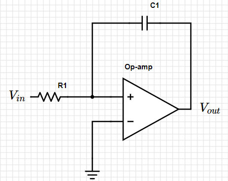Figure 1: Simple integrator circuit. (Image source: Mustahsin Zarif)

Moving into the Laplace domain, we can represent the circuit with the formula:

Vout = -(1/s) (1/RC) Vin

1/s in the Laplace domain actually corresponds to integration! Therefore, we have a circuit model for an integrator circuit using an op-amp. However, when we turn to the real world, systems are always contaminated with some form of random noise.

Putting the integrator circuit on hold for a simpler example, consider a voltage amplifier circuit whose input and output waveforms can be measured with an oscilloscope like Figure 2.

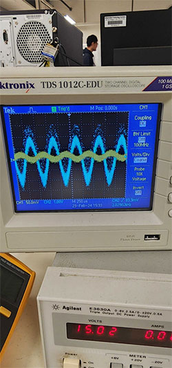Figure 2: Voltage amplifier input and output waveforms. (Image source: Mustahsin Zarif)

The random noise that is added to the underlying, visible sinusoidal waveforms can be owed to a plethora of factors, such as poor electrical connections since the circuit is built on a breadboard. This noise plagues the integrator’s waveform too, which we will see in a future blog in this series on Signal Processing. However, what we are often interested in is how to minimize the random disturbances.

Filtering techniques

Engineers like to overcome these obstacles by employing filtering techniques, which can be classified as either 1) Finite Impulse Response (FIR) Filters or 2) Infinite Impulse Response (IIR) Filters.

FIR filters are so called because the output at any time depends on only the current and previous values of the input, and are not dependent on the past values of the output. Therefore, it has a non-recursive structure with no feedback that can be modeled as Equation 1.

Equation 1: FIR filter example equation. (Image source: Mustahsin Zarif)

The integrator circuit is an example of a FIR filter, because the output is dependent only on the input.

IIR filters on the other hand have feedback, since the output at any time depends on previous outputs as well as the current input. This is modeled as Equation 2.

Equation 2: IIR filter example equation. (Image source: Mustahsin Zarif)

Figure 3 is the block diagram visual representation of an IIR filter, which shows how inputs and outputs are delayed (z-i, z-j), scaled (ai, bj), and summed to give the present output. By changing these values around, we can implement different types of filters.

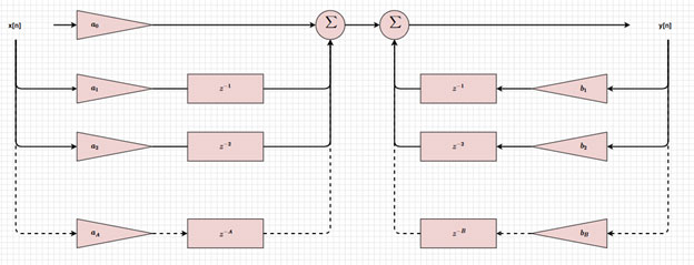Figure 3: Block diagram of an IIR filter. (Image source: Mustahsin Zarif)

If we wanted the block diagram of a FIR filter which has no feedback, y[n] would just be the result of the first summation (Figure 4).

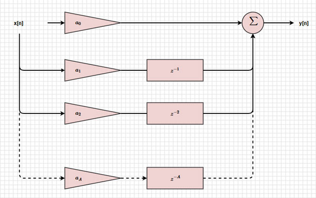Figure 4: Block diagram of a FIR filter. (Image source: Mustahsin Zarif)

Now that we have the basics of FIR and IIR filters down, let’s use an example to illustrate what we learned: the moving average filter.

The way the moving average works is by taking the average of the current input and a certain number of previous inputs (Equation 3).

Equation 3: Moving average equation. (Image source: Mustahsin Zarif)

Where N= window size/number of samples contributing to the output

We can see that this is a FIR filter, since there are no y terms on the right hand side of the equation.

However, we can be smart and rearrange the equation to form an IIR filter. Consider the following:

Let N=5, so

y[5] = (x[5]+x[4]+x[3]+x[2]+x[1])/5,

and y[6] = (x[6]+x[5]+x[4]+x[3]+x[2])/5

y[6]=(x[6]+y[5]-x[1])/5

Therefore, the current output now depends on the previous output (y[6] depends on y[5])!

In more general terms,

y[n] = (y[n − 1] + x[n] − x[n − N - 1])/N

Where N=window size

This filter works wonders in smoothing time-domain signals, as is shown by the Figure 5 which I simulated using python for a window size N = 11.

Figure 5 : Moving filter simulation using Python. (Image source: Mustahsin Zarif)

Moving Filter Simulation Python Code:

Copyimport numpy as np

import matplotlib.pyplot as plt



# Parameters for the sinusoidal wave

frequency = 5  # in Hertz

sampling_rate = 100  # Sampling rate in samples per second

duration = 2  # in seconds



# Generate time axis

t = np.linspace(0, duration, int(sampling_rate * duration), endpoint=False)



# Generate a clean sinusoidal signal

clean_signal = np.sin(2  np.pi  frequency * t)



# Add random, white (Gaussian) noise to the signal

noise_amplitude = 0.5

noisy_signal = clean_signal + noise_amplitude * np.random.normal(size=t.shape)



def moving_average(signal, window_size):

    window = np.ones(window_size) / window_size

    return np.convolve(signal, window, mode='same') 



# Apply moving average to the noisy signal

window_size = 11

smoothed_signal_ma = moving_average(noisy_signal, window_size)



# Plot the noisy and smoothed signals

plt.figure(figsize=(12, 9))



plt.subplot(2, 1, 1)

plt.plot(t, noisy_signal, label='Noisy Signal', color='orange')

plt.title('Noisy Sinusoidal Signal')

plt.xlabel('Time [s]')

plt.ylabel('Amplitude')

plt.grid(True)

plt.legend()



plt.subplot(2, 1, 2)

plt.plot(t, smoothed_signal_ma, label='Smoothed Signal (MA)', color='green')

plt.title('Smoothed Signal using Moving Average')

plt.xlabel('Time [s]')

plt.ylabel('Amplitude')

plt.grid(True)

plt.legend()



plt.tight_layout()

plt.show()

Summary

We began this blog by showing how, in the real world, data is corrupted by noise. While we cannot get the ideal response that we would expect from mathematical equations, it is possible to filter out undesired characteristics from our collected data to match the ideal response as closely as possible. There are multiple methods of doing this, and multiple scenarios where we would want to do so. While we ended this blog with a simulated response of the moving average filter, for the next blog we will look at how the Exponentially Moving Average filter can smooth noisy Inertial Measurement Unit (IMU) data!